Building a Faster Triangular Solver than MKL

A significant part of my research involves investigating algorithms with interesting properties and then trying to optimize them to fully understand how they work. One recent, and fairly successful, exploration was into triangular substitution solvers. In this blog post, I'm going to explain the algorithm and an unconventional recursive approach that broadly abstracts the design space for possible optimizations.

The end result is a lower-triangular (forward substitution) linear equation solver that beats MKL, at least on a (not too) simplified version of the problem. If you just want the sources and none of the story, they are available on GitHub.

For the rest of this article, I'm going to assume you know entry level matrix computations, i.e. how to multiply matrices and vectors, and how to do Gaussian Elimination.

BLAS and triangular solvers

(If you are already familiar with BLAS or with strsv you can skip this section.)

BLAS (Basic Linear Algebra Subprograms) is a specification of an interface of common linear algebra operations, such as (most famously) matrix multiplication, vector fused multiply-adds, and triangular substitution solvers. Most commonly, BLAS-es are implemented in Fortran because of its superior aliasing semantics (the restrict keyword is not necessary), but they are also available in C/C++ through the standard "cblas" interface.

The idea is that by specifying the interface and providing a reference implementation, hardware vendors can produce optimized libraries for each of their architectures. And boy, do they ever! There's a wealth of academic literature and millions of dollars of commercial effort put into optimizing these routines. Among the more notable implementations are OpenBLAS (which is based on GotoBLAS), ATLAS (which tries to automatically tune itself to your hardware), the AMD Optimizing CPU Libraries (aka AOCL), NVIDIA's GPU-based cuBLAS and NVBLAS (which are ridiculously fast), and most famously, there's MKL, which is widely regarded as the gold standard of x86 CPU BLAS implementations (well, at least Intel's x86, though this might be changing). This list isn't exhaustive; supercomputing vendors like Cray supply BLAS-es that are tuned to their hardware.

Now, as I explain in my CppCon 2020 talk, BLAS and high-performance libraries like it are fundamentally limited because they have to synchronize with main memory in between each library call. There's no effective way to fuse computations across stages. There are some C++ libraries, like Eigen and armadillo, that use templates to get some amount of fusion. However, their results are less consistent, and their optimizations are less dramatic (local fusion is no match for global reorganization) than using a full DSL designed for the task, like the Halide language I work on. More on Halide in a future post!

Still, most BLAS-es do a very good job of optimizing their routines. Matrix multiplication in particular is an excellent exercise for anyone interested in understanding machine performance because there are $O(n^3)$ floating-point operations (FLOPS) to schedule against only $O(n^2)$ data. This endows the problem with a very rich design space. In fact, here at UC Berkeley, it is the first assignment in our graduate parallel computing course. If you're interested, the homework materials are here. (By the way, I'm proud to say that while writing this article I learned that my work as a teaching assistant on the Spring 2020 edition of the course earned me an "Outstanding GSI Award" from the EECS department.)

The API that we're discussing today is strsv. The problem it solves is the matrix equation $Ax=b$ where $A$ is a square $n \times n$ matrix, and $b$ is a vector of length $n$. $A$ is assumed to be triangular, which allows fast solving because simple, direct substitution may be used. Here's a quick example; suppose we have the following equation: $Ax = \begin{pmatrix} 1 & 0 & 0 \\ 3 & 1 & 0 \\ 4 & 2 & 1 \end{pmatrix} \begin{pmatrix} x_1 \\ x_2 \\ x_3 \end{pmatrix} = \begin{pmatrix} 1 \\ 1 \\ 1 \end{pmatrix} = b$ Because $A$ is lower-triangular, we can immediately tell that $x_1 = 1$. We can very quickly eliminate $x_1$ in the other rows, by just multiplying $x_1$ by the coefficient in each row in the column and subtracting it from the latter values of $b$. So we'll subtract $3$ and $4$ from the second and third entries to get: $\begin{pmatrix} 1 & 0 & 0 \\ 0 & 1 & 0 \\ 0 & 2 & 1 \end{pmatrix} \begin{pmatrix} x_1 \\ x_2 \\ x_3 \end{pmatrix} = \begin{pmatrix} 1 \\ -2 \\ -3 \end{pmatrix}$

For a quick sketch of a proof of why this works, notice that each row operation is equivalent to a matrix multiplication. In this case, the matrices $R_1, R_2$ (below) applied to both sides of the equation (on the left, since matrix multiplication is not commutative), gives us the equation we have above.

$R_1 = \begin{pmatrix} 1 & 0 & 0 \\ -3 & 1 & 0 \\ 0 & 0 & 1 \end{pmatrix} \; R_2 = \begin{pmatrix} 1 & 0 & 0 \\ 0 & 1 & 0 \\ -4 & 0 & 1 \end{pmatrix}$

That is, the equation $Ax = b$ has the same solution as $(R_2 R_1) A x = (R_2 R_1) b$.

In the final step, we eliminate the second column: $\begin{pmatrix} 1 & 0 & 0 \\ 0 & 1 & 0 \\ 0 & 0 & 1 \end{pmatrix} \begin{pmatrix} x_1 \\ x_2 \\ x_3 \end{pmatrix} = \begin{pmatrix} 1 \\ -2 \\ 1 \end{pmatrix}$ We can check this answer, too: $Ax = \begin{pmatrix} 1 & 0 & 0 \\ 3 & 1 & 0 \\ 4 & 2 & 1 \end{pmatrix} \begin{pmatrix} 1 \\ -2 \\ 1 \end{pmatrix} = \begin{pmatrix} 1 \\ 1 \\ 1 \end{pmatrix} = b$

Hooray! In the next section we'll go over the algorithm in the abstract and write a naive implementation.

Solver algorithm and interface

So what does this look like as a formal algorithm? Well, what did we do on paper? We started by going across the columns, and then within each column, using the newly solved value in $x$ to update the unsolved part. As a "plain" English algorithm, it looks like this:

1. Solving: $Lx = b$
2. Set $x = b$
3. For each column $j$ of $L$:
   1. Set $x_j \leftarrow x_j / L_{jj}$.
   2. For each row $i$ in the column $j$, starting with $j+1$:
      1. Update $x_i \leftarrow x_i - x_j \cdot L_{ij}$

Now how do we turn this into code? For the sake of space (and my sanity writing and optimizing this stuff), we'll make the following simplifying assumptions:

1. The matrix $L$ is lower triangular.
2. The matrix $L$ has all $1$s on its diagonal. This lets us skip the division on line (3.1) above.
3. The matrix $L$ is stored in column-major order.
4. The matrix $L$ is stored in a large, dense array in natural order; the upper half might contain useful information (like an upper triangular matrix), so we cannot overwrite it or assume it to be zero.
5. The vector $b$ is stored in a normal array and may be overwritten with the solution $x$.
6. We're running on a single CPU core.

The naive translation under these assumptions into plain C is this:

1
2
3
4
5
6
7

void naive_solver(int n, float* L, float* x) {
  for (int j = 0; j < n; ++j) {
    for (int i = j + 1; i < n; ++i) {
      x[i] -= x[j] * L[i + n * j];
    } 
  } 
}

These assumptions are so common that the BLAS API for this takes extra arguments to inform the implementation when these are the case. Here's the full signature in C:

1
2
3
4
5
6
7
8
9

enum CBLAS_ORDER {CblasRowMajor=101, CblasColMajor=102};
enum CBLAS_TRANSPOSE {CblasNoTrans=111, CblasTrans=112, CblasConjTrans=113};
enum CBLAS_UPLO {CblasUpper=121, CblasLower=122};
enum CBLAS_DIAG {CblasNonUnit=131, CblasUnit=132};

void cblas_strsv(const enum CBLAS_ORDER order, const enum CBLAS_UPLO Uplo,
                 const enum CBLAS_TRANSPOSE TransA, const enum CBLAS_DIAG Diag,
                 const int N, const float *A, const int lda, float *X,
                 const int incX);

The name strsv encodes a few facts about the function. The leading s stands for "single-precision" and the trailing v stands for "vector". The base name of the function is therefore trs, which is short for "triangular solve". Thus, the function solves a triangular matrix-vector equation in single precision (i.e. float).

The order argument determines whether the input matrix will be treated as row major or column major. To be column-major simply means that adding 1 to the pointer into the matrix will move down one row (ie. with the current column); similarly, row-major means that adding 1 moves to the right one column. The Uplo argument tells the implementation whether we're giving it a lower or upper triangular matrix. The TransA algorithm allows the user to ask that BLAS implicitly transpose (or conjugate transpose in the case of complex values) while solving. Finally, the Diag argument tells strsv whether the main diagonal is all 1s.

So we can implement a function with the same signature and contract as above using the BLAS library like so:

1
2
3
4

void blas_solver(int n, float* L, float* x) {
  cblas_strsv(CblasColMajor, CblasLower, CblasNoTrans, CblasUnit,
              n, L, n, x, 1);
}

Now is a good time to benchmark these two implementations to get some idea of how far off we are.

Benchmarking setup

First things first: we need to understand how much work we're doing. It's pretty clear that we're doing $O(n^2)$ operations, but it's easy enough to get an exact count. If we look at the naive algorithm, we'll notice that the innermost update consists of two floating-point operations: (1) the multiplication between x[j] and L[i + n * j], and (2) the subtraction of the resulting value from x[i]. Then the inner loop runs between $j+1$ (inclusive) and $n$ (exclusive). That's $n-j-1$ iterations in total. The outer loop runs between $j=0$ to $j=n-1$. In math terms, the total number of FLOPS is:

$2 \cdot \sum_{j=0}^{n-1} n-j-1 = 2 \cdot \sum_{j=0}^{n-1} j = 2 \cdot \frac{n \cdot (n-1)}{2} = n \cdot (n-1)$

So to solve an instance with an $n\times n$ matrix, we must perform $n\cdot (n-1)$ floating-point operations.

We're going to use AVX2 to optimize this routine because it's still a bit more widely available than AVX-512 (and because it doesn't have quite so extreme CPU frequency offsets). I have benchmarking set up on GitHub Actions. At time of writing, the cloud runners have Xeon 8171M CPUS clocked down to 2.3GHz. I also tested locally on my i9-7900X workstation. Both CPUs are Skylake, so I compile with -march=skylake on GCC.

We're going to test against both OpenBLAS and MKL. By default, both BLAS-es dispatch the APIs to hardware-specific implementations by sniffing CPU flags. Since the GitHub Actions runners support AVX-512, this would pose a challenge. Fortunately, both BLASes offer ways to override this. When compiling OpenBLAS, we may set -DTARGET=HASWELL on the CMake command line. For MKL, we can run export MKL_ENABLE_INSTRUCTIONS=AVX2. To keep things on one core, we can export OPENBLAS_NUM_THREADS=1 and link to the sequential MKL library.

To get a full picture of performance, we'll test on a variety of matrix sizes so that we can see how we perform when the data fits inside L1, L2, or L3 cache, plus when it spills out into RAM. The L3 cache of the GitHub Actions chips is 35.75MB in size. Without getting too much into the math, there's 4 bytes per float and less than $n^2$ data in our working set. So using matrices at least as large as $3000\times 3000$ will exceed L3. To be safe, we'll use $n=4096$ as the upper bound.

Finally, I'll use Google Benchmark to compute performance numbers and use the formula we derived above to scale raw time into FLOPS.

So here's our baseline:

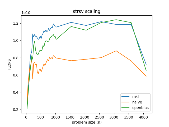
Keeping in mind that GCC has already auto-vectorized the naive implementation, there doesn't seem to be a lot of headroom here. Roughly speaking, it looks like the naive solutions runs at about 8 GFLOPS, while MKL runs around 12 GFLOPS or 50% faster. OpenBLAS is generally slower, but seems to do slightly better than MKL when the size of the matrix is just about to escape the computer's L3 cache. Naturally, once we hit RAM, the $O(n^2)$ work just isn't enough to hide the latency of the $O(n^2)$ memory. This is in stark contrast to matrix multiplication, which has $O(n^3)$ work to do.

A curious recursion

While analyzing the algorithm, I made one key observation: at the start of the inner loop on iteration $j$ of the outer loop, all the values of $x_i$ for $i \leq j$ are finalized. Thus, we can reformulate the problem into a recursive algorithm that solves the top $k \times k$ triangle first, then uses the first $k$ entries of $x$ along with the $n-k \times k$ rectangle below that triangle to update the remaining $n-k$ entries of $x$. Finally, we can solve the right $n-k \times n-k$ triangle with the updated bottom part of $x$.

This is a sort of divide and conquer approach to this problem. When I came up with it, I had never seen it before, but when I started poking around, I found some recent work by Elmar Peise and Paolo Bientinesi: "Recursive Algorithms for Dense Linear Algebra: The ReLAPACK Collection". On the one hand, this was disappointing because my idea wasn't actually novel (hence, a blog post rather than a research paper); on the other hand, this was encouraging because it meant I was on the right track. Such is life.

Anyway, the next insight is that the way you combine the lower rectangle with the solved part of $x$ is to compute a matrix-vector product between them and subtract the result from the unsolved part of $x$. To see that, look at the computation we're doing:

x[i] = x[i] - L[i, j] * x[j]

Now $j$ ranges over $[0, k)$, because we already handled the top triangle. We also know that $i$ ranges from $k$ to $n$. This code then becomes the following, in numpy-esque vector notation:

x[k:n] = x[k:n] - L[k:n, 0:k] * x[0:k]

Very helpfully, the BLAS contains an operation, sgemv, that does exactly this. So the lazy way to implement the recursive algorithm is to reduce it to sgemv like this:

 1
 2
 3
 4
 5
 6
 7
 8
 9
10
11
12
13
14
15
16
17
18
19
20
21

void solve_dnc(int n, float *L, int lda, float *x) {
  if (n <= BASE_CASE_LIMIT) {         // Naive algorithm.
    for (int i = 0; i < n; ++i) {     // GCC happens to generate better code
      for (int j = 0; j < i; ++j) {   // for this loop order. Don't know why.
        x[i] -= x[j] * L[i + j * lda];
      }
    }
  } else {
    int k = n / 2; // WOAH - this one line determines the algorithm

    // Upper triangle -- reads L(:k,:k), x(:k); writes x(:k)
    solve_dnc(k, L, lda, x);

    // Rectangle -- reads L(k:,:k), x(:k); writes x(k:)
    cblas_sgemv(CblasColMajor, CblasNoTrans, n - k, k, -1.f, L + k, lda,
                x, 1, 1.f, x + k, 1);

    // Right triangle -- reads L(k:,k:), x(k:); writes x(k:)
    solve_dnc(n - k, L + lda * k + k, lda, x + k);
  }
}

This version takes an extra parameter, lda, to manage the distance between columns independently of the logical dimension. The neat thing about this characterization is that it lets us explore the space of optimizations entirely by varying the function that calculates $k$. In this case, we chose a recursive approach, but we could also set it to, say, BASE_CASE_LIMIT to proceed in blocks of columns (spoiler alert!), or to n - BASE_CASE_LIMIT to proceed in blocks of rows. Various hybrid approaches could be designed off of this, too, all by varying that one line of code.

There are some clear disadvantages here. This isn't tail recursive, so it will take some extra stack space and cost some function call overhead. The compiler also can't inline strsv since it's squirreled away in a shared library and is very, very proprietary (so no-go on LTO). Still, this exercise has clearly exposed our best vectorization opportunity. It would be very difficult to vectorize a small triangle, but maybe we can get away with only doing $O(n)$ serial triangles, and $O(n^2)$ easier-to-vectorize rectangles.

Since I know you're curious, this is how well the $n/2$ divide and conquer approach works.

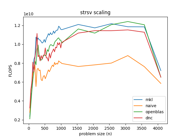
It's surprisingly in the ballpark when using OpenBLAS's sgemv. What's interesting is that for at least one matrix size, it ever-so-slightly edges out MKL, despite being built from OpenBLAS. This could be a fluke, but I bet there's an even better optimization than any in this article that we just haven't found yet.

Lower-level optimization

I played around with the divide-and-conquer approach for a bit and settled on a split "function" of simply $k=8$. That corresponds to looping over 8-wide block columns of the matrix, solving the $8\times 8$ triangle at the top and then the whole rectangle beneath it. It seemed to perform best on my workstation, and so I set out to "inline" everything and get it cleaned up. Here it is, chunk by chunk.

Note, for simplicity, I'm specializing this code to multiple-of-8 matrix sizes. Extending it to other matrix sizes only requires dealing with a small leftover rectangle at the bottom of each block column. It's just another code path, and the same basic strategies apply. It's a good exercise, but too much for a blog post. Also, as you'll see, the resulting code is so much faster that MKL could get a boost just by testing the matrix size and then dispatching to this solver if it fits. That one branch up front would cost next to nothing.

First, we'll declare the function and start looping:

void update_blocked(int n, const float *L, int lda, float *x) {
  while (true) {

So why are we using an infinite loop here rather than a for loop over the block columns? Well, remember that we're going to solve a triangle, then a rectangle, then a triangle, and so on until we hit the rightmost triangle, which has no rectangle underneath it. So we want to exit the loop right away without testing the conditions for the would-be for loop or for the rectangle code again. Here's the code for the triangle and early stopping:

    // Handle triangle at top of block column
    for (int j = 0; j < 8; ++j) {
      for (int i = j + 1; i < 8; ++i) {
        x[i] -= x[j] * L[i + lda * j];
      }
    }

    n -= 8; // Last iteration doesn't have a rectangle
    if (n <= 0) { return; }

At this point, we have solved the first 8 values of $x$. We subtract 8 from $n$ right away since the following code operates on the shorter rectangle. Now we're going to take those 8 values we just computed and broadcast them into 8 vector registers. We first create a typedef to use GCC's vector types feature,

// Vector of 8 single-precision floats
typedef float v8sf __attribute__((vector_size(32), aligned(1)));

and then create an array of these with the broadcast values:

    v8sf x_solved[8];
    for (int i = 0; i < 8; i++) {
      x_solved[i] = _mm256_broadcast_ss(&x[i]);
    }

Because we're using GCC's vector types and its own intrinsics, it is smart enough to compile this into exactly 8 instructions that load the values into registers. So there's no overhead from the loop or from the array. We load these values into registers now because they're involved in every computation in the rectangle, so we don't want to constantly reload them from memory. We broadcast them so that we can load individual columns into vectors from inside the block column. For example, we can take a vector from the first column in the block, multiply it by x_solved[0] and then subtract it from the corresponding portion of x.

To set this up, we'll advance L to point to the top of the rectangle and advance x to point to the first unsolved portion and then enter the loop:

    L += 8;
    x += 8;

    for (int i = 0; i < n; i += 8) {

The first order of business is to load a vector's worth of the unsolved chunk of x. We have to do an unaligned load (loadu) because alignment wasn't in our assumptions and because aligning it would take too long (remember, $O(n^2)$ on both operations and memory).

      v8sf x_i = _mm256_loadu_ps(&x[i]);

Then we'll load an $8 \times 8$ patch of $L$ into vectors using the same trick as above.

      v8sf L_patch[8];
      for (int j = 0; j < 8; j++) {
        L_patch[j] = _mm256_loadu_ps(&L[i + lda * j]);
      }

Finally, we update the unsolved vector using that patch of values from the matrix. We write the vector back to x and advance L to the tip of the next triangle, ready to repeat the process.

      for (int j = 0; j < 8; j++) {
        x_i -= x_solved[j] * L_patch[j];
      }

      _mm256_storeu_ps(&x[i], x_i);
    } // for i

    L += lda * 8;
  } // while true
}

The assembly generated for the rectangle loop is as short as can be. Just thirteen instructions, almost all vectorized. You can see the full assembly on Godbolt, here: https://godbolt.org/z/YGWfoz9fs.

 1
 2
 3
 4
 5
 6
 7
 8
 9
10
11
12
13

.L5: vmovups ymm0, YMMWORD PTR [r8+32+rax*4]
     vfnmadd213ps    ymm0, ymm8, YMMWORD PTR [rsi+32+rax*4]
     vfnmadd231ps    ymm0, ymm7, YMMWORD PTR [r15+32+rax*4]
     vfnmadd231ps    ymm0, ymm6, YMMWORD PTR [r14+32+rax*4]
     vfnmadd231ps    ymm0, ymm5, YMMWORD PTR [r13+32+rax*4]
     vfnmadd231ps    ymm0, ymm4, YMMWORD PTR [r12+32+rax*4]
     vfnmadd231ps    ymm0, ymm3, YMMWORD PTR [rbx+32+rax*4]
     vfnmadd231ps    ymm0, ymm2, YMMWORD PTR [rdi+32+rax*4]
     vfnmadd231ps    ymm0, ymm1, YMMWORD PTR [rcx+32+rax*4]
     vmovups YMMWORD PTR [rsi+32+rax*4], ymm0
     add     rax, 8
     cmp     r9d, eax
     jg      .L5

The beauty of this is how it minimizes memory traffic. We're streaming memory in from $L$ exactly the one time we need it, as part of the instruction that needs it. In the assembly above, ymm0 stores the unsolved vector from $x$, while ymm1-8 store the broadcast solved values.

The code for the triangle is messy and mostly scalar, but I stopped trying to optimize once I saw this:

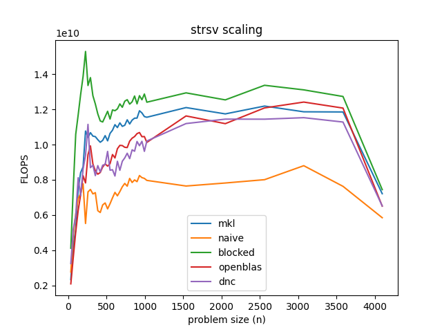
At least on GitHub Actions, this blocked solver is never slower than MKL. At peak, it's nearly twice the speed of the naive solver and 50% faster than MKL, roughly. This is why I said I didn't want to bother with non-multiple-of-8 sizes earlier. The dispatch would be totally lost in the gap.

Conclusion

The triangular solver routine must not get a lot of love in BLAS implementations. Judging by the performance of my divide and conquer solver, I wouldn't be surprised if MKL and OpenBLAS were just using (an inlined version of) their own sgemv routines without giving this one any special attention. Still, the results to effort ratio here is pretty striking.

It would be an interesting exercise to build a full-strength solver that handles all matrix sizes, row-major layouts, double precision, etc. but that's too much for one blog post (and too much for my purposes of understanding the design space of this algorithm better).